Guest post: Avery Cutler is a senior at Bowdoin College, double majoring in Mathematics and History with a minor in Urban Studies. She is interested in quantitative analyses of housing structures and insecurities, and she hopes to continue exploring urban sciences through research opportunities that focus on thoughtful understanding and community-impact.
This analysis works to understand potential predictors and patterns in US housing unit count growth data from 2020-2025. The most recent housing count record from 2025 considers more detailed, accurate, and timely data than the US Census can provide. Through these analyses, I hope to provide quantitative insight into what concrete changes will have influential factors on housing units, and subsequently, household counts. More generally, this project produces a preliminary understanding of the influence that various demographic factors have on housing unit counts at the county level. With a higher processing computer, the same workflow can be completed with census tracts or other more granular geometries.
By implementing a Bayesian framework, this exploration considers uncertainty as an inherent contributor of the output distribution. For this specific exploration, the model considered a normal distribution of error centered around 0 for each input regressor. Consequently, the output of our model hypothesizes a distribution of values that include possible coefficients of our model and builds predicted value outcomes. When a coefficient distribution contains 0, we anticipate that the impact that this regressor has on our model may not be influential. This modeling technique also allows us to estimate changes to the posterior distribution of housing unit growth through posterior draws and subsequent manipulation.
The following findings detail regressors that, through our model, have confident influences on housing unit counts. Furthermore, by considering the model’s posterior estimates, I developed a function that considers how changes in the regression input could output a different expected housing unit change distribution. This interactive element is helpful in determining what changes will influence housing unit counts more than others. An important caution with this model is that these relationships might not be explicitly causal and should not be treated as such.
Preliminary modeling
In addition to exploring vacancy percentages and household growth data through Bayesian techniques, the bulk of my exploration considered housing units as the dependent variable. After initially considering tract level geometries, I focused my exploration to counties. This exploration considered variables from the following Census and LEHD Origin-Destination Employment Statistics (LODES) Dataset categories: median income, renting percentage, standardized 2020 county population, median home value, county racial demographics, county citizenship demographics, wage changes from 2015 to 2020, vacancy percentage (excluding second homes), percentage experiencing poverty, and initially around 50 job categories from the LODES dataset. This last section was ultimately trimmed down to 28 variables using an exploratory data analysis process. After collinearity checks, this model ultimately considered 42 predictive variables of housing unit growth from 2020 to 2025.
In this dataset containing over 3000 US counties, only 18 of them had negative or zero housing unit growth. For the sake of modeling accuracy, I removed these counties from the analysis. The codes for those counties are listed as follows: 02013, 02016, 02050, 02066, 02070, 02100, 02105, 02158, 02164, 02180, 02185, 02188, 02240, 02275, 02282, 15005, 48261, 48301. After this cleaning, I Winsorized my outliers: a standard outlier transformation technique used for model fitting ease that redefines all datapoints whose outcome is greater than the 95th percentile value to that upper-value limit. After this transformation, I applied a gamma distribution to fit the positive, rightly-skewed housing unit counts histogram. In an exploratory modeling phase, I considered a linear regression to predict changes in the model considering all of the above regressors. The linear regression showed predictive power and potential, but the fit increased with the gamma model. The output of that model can be found here. Consequently, for the Bayesian exploration, I continued to use a gamma fit.
Bayesian exploration
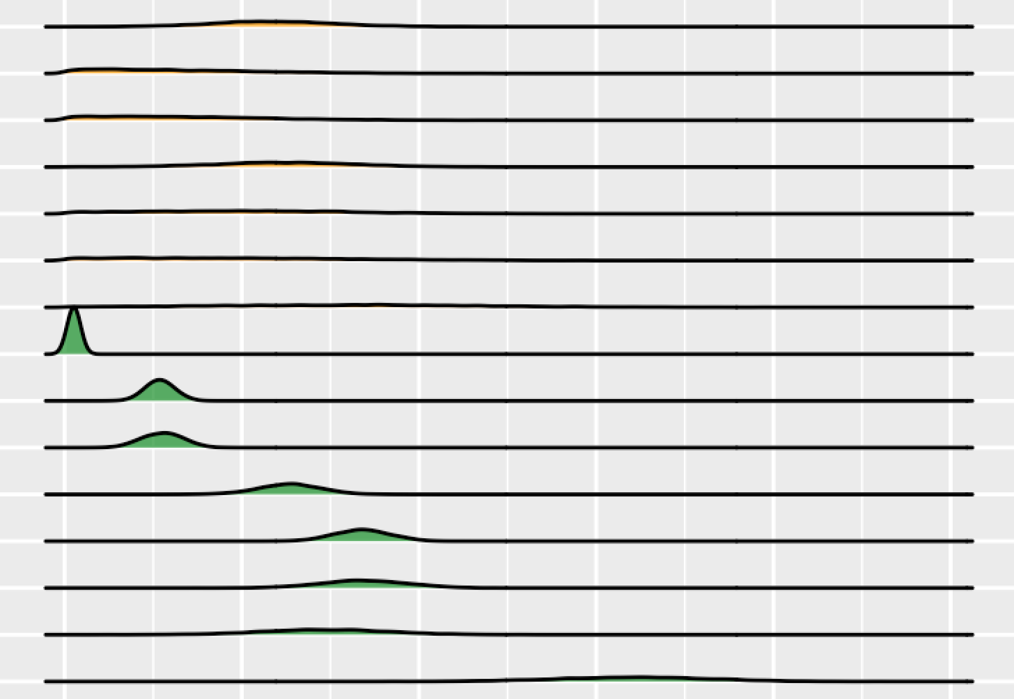
After running 42 variables in the Bayesian regression, the model determined distributions of all of the regressor coefficients and determined an estimated posterior distribution. A visualization of the coefficient distributions are found in the density plots below. The variables that did not contain 0, and thus confidently influence the housing unit count outcome, are shown in green in the chart. The second graph shows the absolute values of all regressor coefficient distributions in ascending order and stratified by if they contain 0. The last visualization shows the coefficient distributions that do not contain zero, and their numeric summaries are in the chart that follows.

| Variable | Min | 1st Qu. | Median | Mean | 3rd Qu. | Max |
|---|---|---|---|---|---|---|
| Percentage of the population that is white | −2.645 | −1.711 | −1.468 | −1.470 | −1.229 | −0.045 |
| Standardized wage change from 2015–2020 | 0.258 | 0.484 | 0.538 | 0.538 | 0.590 | 0.825 |
| Vacancy percentage (excl. second homes) | −2.028 | −1.386 | −1.271 | −1.267 | −1.151 | −0.587 |
| Percentage of homes that are rented | −2.252 | −1.782 | −1.678 | −1.677 | −1.572 | −1.179 |
| Jobs in NAICS 11 (Agriculture, Forestry, Fishing & Hunting) | −0.098 | −0.061 | −0.052 | −0.052 | −0.043 | −0.002 |
| Median income in county | −1.025 | −0.630 | −0.554 | −0.551 | −0.471 | −0.123 |
| Jobs with earnings $1,251–$3,333/month | 0.742 | 1.527 | 1.685 | 1.688 | 1.851 | 2.439 |
| Model intercept | 1.532 | 2.916 | 3.216 | 3.207 | 3.498 | 4.634 |
In addition to these coefficient outputs, I modeled posterior predicted values to simulate the housing unit growth distribution based on our model. This distribution comparison is seen in the histogram below.

Using this synthetic data, I developed a function that considers alterations in the seven significant regressors and outputs how the posterior distribution may be expected to change. For example, the density distribution below is what is expected of the housing counts across the nation when the standardized number of jobs with earnings $1251/month to $3333/month decreases to 25% of its current value. This depicts the relationship between some lower paying jobs being offered at a high rate and fewer housing units growing. This tool can be manipulated in various ways to show numerous variable changes or specific regressor changes independently.

Additional findings and next steps
In addition to building this model, I considered the potential influence of spatial autocorrelation on housing unit growth for various counties. Before implementing a spatial component to the Bayesian analysis through a spatial prior, I used a Global Moran’s I test to test the hypothesis that there is a random distribution of housing unit growth increase across adjacent and nonadjacent counties. After building a county adjacency matrix from Census data, I found a p-value of < 2.2e-16 which rejects the possibility that there is random spatial structure. This finding motivates the implementation of a Spatial Autoregressive Model to better fit housing unit count growth. The results of this model would consider county proximity to counties with increasing housing unit counts as a potential contributor to each county’s own housing unit growth. The gamma regression from this past exploration would be considered alongside a matrix defining county proximities, and the output coefficients of this model may vary from the nonspatial due to the new predictive considerations.
Ultimately, this exploration provided a baseline understanding of how housing unit counts can be modeled and predicted across US counties. This research could be helpful in determining present day household counts, a statistic that is not readily available but could be determined through “now-casting”-like analyses. More generally speaking, Bayesian explorations of housing unit count data provide meaningful avenues for understanding the interaction of potentially influential demographic qualities on housing realities and discrepancies across the nation.
Thank you to Avery Cutler for the research and guest post.